1. INTRODUCTION
The decision to implement port projects requires large investments, therefore, it is necessary to map the risks and uncertainties inherent to the technical, economic and environmental feasibility of the enterprise. The strategic location of the State of Pará as a logistics warehouse for the world, leads to the search for a strategic port solution to enhance the logistics vocation that the State has, aiming to benefit the northern region and Brazil in general.
A preliminary study will be able to predict the main risks and uncertainties that may occur with the implementation of the project and determine if there is feasibility of its construction, and if is, what are the main risks that will need to be foreseen during the execution phase of the project and in the period where it is already operating. The implementation of an offshore port in the north of Brazil, in addition to accompany the evolution of the naval industry, with the increase in the size of ships, it will enhance the use of the main output of cargo from the 'northern arc', reducing the cost of Brazilian freight. (MORAES, et al. 2017)
The northern region of the country, with exclusive focus on Pará, comes across as geographically privileged due to its proximity to the main canal used in trade routes (Panama Canal) and the fact that 70% of the maritime comercial routes travel through the north hemisphere (MORAES, et al. 2017).
Aware of the logistical potential that the State of Pará has, this article aims to analyze the risks of implementing an offshore port in the north of the State, through a risk analysis software that uses the Monte Carlo methodology to obtain its results.
To fulfill the main objective of the article, the following specific objectives were assigned: Develop a model for risk analysis; Perform risk analysis using @RISK software; and evaluate the feasibility of implementing the port project.
2. LITERATURE REVIEW
2.1 Alternative and logistics for cargo transportation in Brazil
The aptitude for the use of waterway transport in Brazil, despite being an obvious choice, has been overlooked with a clear preference to the road transportation, with more investments, however, this mode has a high added value of freight when compared to the waterway mode by its low load capacity and high energy consumption (FERREIRA; RIBEIRO, 2002).
This preference of transportation mode is detrimental to the northern region of Brazil because road freight to the region is more expansive. The logistics of the northern region is the most viable for the country due to its position close to the large consumer markets, however, to make this logistical advantage viable in the North of the country, it is necessary to build a port connected with the main ports in the world in terms of ship size and technology (LOPEZ; GAMA, 2007).
2.2 Elements for a project analysis
For the evaluation of a project, four elements are involved in which they are correlated with each other, meaning that all these elements are necessary to obtain a complete analysis of the project, among them are listed
- Technological aspects mainly deal with the technical processes of project construction and its operation when completed, as well as capital and operating cost estimates. (ADLER, 1978)
- The administrative assessment refers to the numerous management and staffing problems that arise in construction and operation. (ADLER, 1978)
- Financial analysis acts on expenses and revenues, that is, verifying if the project is financially viable, if it generates a reasonable return on the invested capital. They are usually summarized in the company's cash flow statements and balance sheets. (ADLER, 1978)
- Economic evaluation focuses on measuring its costs and benefits from the point of view of a country as a whole. (ADLER, 1978)
The risk model set up for the application of the @RISK program calculates the benefits, revenues, operating costs, construction costs and administrative costs over a period of thirty-five years, using the program will aid to visualize the year and the event which will have more impact on variable values, such as project benefits and revenues, thus performing the analysis in the form of graphics, facilitating decision making if the project proves itself viable or not.
2.3 Monte Carlo Method (MCM)
Monte Carlo Simulation (MCS) is a statistical simulation method that can be defined as a methodology that uses a sequence and random numbers to generate a simulation. (SOUZA, 2004).
The first author to illustrate the applicability of Monte Carlo simulation was David Hertz, in his article Risk Analysis in Capital Investment, published in 1964. The article emerged with the use of Monte Carlo Simulation in project analysis, as a way of measuring the risks inherent to each variable.
Nowadays, the MCS is widely used to perform market analysis for possible investments, due to its ability to reveal the possible risks and uncertainties present in the investment (HERNANDEZ, 2012). There are risk analysis softwares based on MMC, for example, @RISK.
According to Ávila (2015), the Monte Carlo methodology has a guideline to its implementation, defined as:
1° step: Algorithm assignment, to perform the analysis of the desired scenarios and evaluate the probabilities of success or failure;
2° step: Recognition of the scenario to be used and problem modeling;
3° step: Generate random values for the uncertainties surrounding the desired design;
4° step: The uncertainties applied are replaced by the values assigned in order to calculate the results; and
5° step: Obtain an estimate for the solution of the problem based on the analysis of the previous topics.
2.4 @RISK for project risk analysis
According to Cotterell (2016, p. 30) “All projects involve risk, but it's vital to understand what those risks are and how they can affect your budget and schedule. @RISK is a well-established software tool that is designed to help you do this’’.
The chosen software @RISK is considered a Microsoft Excel complement that allows us to analyze risk using the Monte Carlo method. The program can be used to analyze various risks in which it shows virtually all possible outcomes for any situation and indicates the probability of a specific event occurring, so you can analyze which risks to avoid. This risk analysis tool makes everything easier when executing a specific project, as it is an easy-to-learn tool and presents a wide variety of distributions to be used. It still has within the software the specific explanation of the distribution, clearing doubts about the use of each one, thus becoming a great tool for study. This program is used by large companies such as Boeing, Petrobras, Disney, AT&T, NASA, Toyota among others (PALISADE, 2019). It is noticed that the companies that use this tool are from totally different branches, thus showing the great diversity of risk analyzes that can be done with @RISK.
@RISK simulates through the Monte Carlo method the analysis of different types of existing risks and the probability of occurrence. These simulations are performed using a computerized mathematical technique that is based on random sampling capable of calculating the probability of events. With the numerical result of these simulations, it is possible to identify the main project risks and help in decision making.
The program allows us to perform sensitivity analysis of the generated problem, through the definition of inputs and outputs (fixed and variable costs). After creating a risk model, it generates distribution and tornado graphs, where they show us the main values that influence the analyzed project.
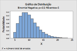
Graph 1 – Example of Distribution Graphic
Fonte: Minitab (2019).
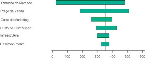
Graph 2 – Example of Tornado Graphic
Fonte: Mauro Sotille (2016).
3. Methodology
Moraes et al. (2017) idealizes an offshore port located in Curuçá at the mouth of the Marajó River, a location chosen because the rest of the coast does not have the necessary conditions to serve large ships and is located outside the limits of environmental reserves, as is the case of the Reserve Great Mother of Curuçá.
The area, according to Moraes et al. (2017), calculated to the project’s structure is a total of 11.136 square meters.
To obtain the results and answers about the problematization presented in this work, a risk analysis will be carried out on the variables through explanatory research with data obtained from primary and secondary sources. Thus, it is possible to develop the risk model, carry out the analysis through the @RISK program and analyze the feasibility of the port project as proposed.
To start the risk model used in @RISK, it is necessary to have a risk model, therefore, research was carried out on the websites of CDP (Companhia docas do Pará), ANTAQ (National Agency for Waterway Transport) and SINAPI 2018 Thus obtaining the necessary information to create this model.
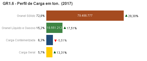
Graphs 1 and 2 show the amount of each cargo in tons that was handled during the given year in the northern region. The values obtained for the spreadsheet, the amount of solid and liquid bulk handled, is the average, in tons, from 2010 to 2018, only in the northern region. The number of containers was taken from the sum of the movement during 2018 in the north and northeast region, plus a 50% increase in the quantity, imagining that this port will concentrate loads for redirection to other Brazilian regions. The port tariffs used in the model were taken from the database of the Companhia de Docas do Estado do Pará and the National Agency for Waterway Transport.

Graph 3 – Cargo handling in the northern region in 2017
Fonte: ANTAQ, 2018
Graph 4 - Cargo handling in the northern region in 2018.
Fonte: ANTAQ, 2019.
The model will be based on the first 35 years of the offshore port, in which the values obtained will serve as a basis for the calculation of the NPV (net product value) of the project, which the program will use as a fixed value for the initial calculation and from that value to simulate the variations.
The variation obtained from the movement of containers used to carry out the risk model was, in the worst case, 500,000 units and 2,500,000 units in the best case. The northern region, according to the ANTAQ yearbook in 2018, handled 427,845 units, and the northeast region 719,259. Considering that the port will benefit not only the north and northeast region but the country as a whole, it was selected as a fixed value 1,500,000 units model. The fixed values for solid and liquid bulk were obtained by the average of movements in tons per year in the ANTAQ’s yearbook of the northern region, in which the fixed value for solid bulk was 60,000,000 tons, where the worst case is 40,000,000 tons and best case of 80,000,000 tons, for liquid bulk it was 15,500,000 tons, with worst case of 13,000,000 tons and best case 17,000,000 tons.
With this base, a spreadsheet was created containing the values acquired, identifying the project's fixed and variable costs, setting up a projection for 35 years. This risk model built in Excel is the basis on which the @RISK program will mount its simulations and will demonstrate in tornado graph forms an aid in decision-making processes, in which it evaluates which variables most impact a project, making it possible to create a plan of action. In this case, it will show which variable and in which year it will have the greatest impact on the NPV (Net Present Value) of the project. It will also have the distribution chart in which it will show if the project of an offshore port in the north of Brazil will be viable or not.
After applying the risk model in the program, it will be necessary to choose the correct distribution to be used in the variable inputs and to use the program tool "Achieve Goal" to identify the best market rate for the model, after analyzing the distributions for the inputs, it will be necessary to mark the output which, in this case, will be the NPV of the model.
The “Achieve Goal” is a tool of fundamental importance, considering that it will give us the maximum rate so that the project’s NPV does not become negative, that is, it eliminates one of the variabilities to be analyzed, demonstrating a more favorable scenario within the conditions established inside the tool.
With the outputs and inputs correctly selected, the program will be able to perform several simulations. In this case, there were ten thousand simulations. When finished, @RISK will show graphs containing the data needed to evaluate the proposed project.
4. Results and Discussion
Data were taken from SINAPI 2018 to obtain the cost of building the port as shown in Table 1, average cargo movement in ports in the northern region and port tariffs appropriate for the project.
Table 1- Project’s costs of construction
|
BUDGET OF REFERENCE – TOTAL INVESTIMENT (construction) |
|||||||
|
ITEM |
DESCRIPTION |
CONSTRUCTION OF THE CONTAINER TERMINAL AND ADMINISTRATION |
CONSTRUCTION OF THE AGRICULTURAL SOLID BULK
|
CONSTRUCTION OF THE MINERAL SOLID BULK TERMINAL
|
CONSTRUCTION OF LIQUID BULK TERMINAL |
TOTAL |
INCIDENCE |
|
|
|
|
|
|
|
(A1+B2+C3+d) |
|
|
|
|
A |
B |
C |
D |
|
|
|
1 |
PRELIMINARY SERVICES |
6.899.011,64 |
4.311.882,28 |
3.018.317,60 |
3.018.317,60 |
17.247.529,12 |
1,03% |
|
2 |
HYDRAULIC LANDFILE |
28.786.514,87 |
19.191.009,91 |
23.988.762,39 |
23.988.762,39 |
95.955.049,56 |
5,72% |
|
3 |
CONTENTION WORKS |
12.810.726,52 |
8.540.484,35 |
10.675.605,43 |
10.675.605,43 |
42.702.421,73 |
2,55% |
|
4 |
ROAD INFRASTRUCTURE |
8.422.509,15 |
8.422.509,15 |
5.615.006,10 |
5.615.006,10 |
28.075.030,50 |
1,67% |
|
5 |
FOUNDATIONS AND STRUCTURES IN REINFORCED AND PRESTRESSED CONCRETE |
321.989.687,43 |
214.656.791,62 |
268.324.739,53 |
268.324.739,53 |
1.073.295.958,11 |
63,99% |
|
6 |
BUILDINGS AND WORKS OF ART |
13.996.652,65 |
1.999.521,61 |
1.999.521,80 |
1.999.521,80 |
19.995.217,86 |
1,19% |
|
7 |
ELECTRICAL AND AUTOMATION INSTALLATIONS |
11.113.828,82 |
6.350.759,20 |
7.144.604,10 |
7.144.604,10 |
31.753.796,22 |
1,89% |
|
8 |
HYDROSANITARY INSTALLATIONS |
376.542,17 |
2.043.738,38 |
2.299.205,68 |
2.299.205,68 |
7.018.691,91 |
0,61% |
|
9 |
FIRE FIGHTING SYSTEM |
1.755.826,70 |
1.003.329,58 |
1.128.745,78 |
1.128.745,78 |
5.016.647,84 |
0,30% |
|
10 |
PORT EQUIPMENT |
1.058.000,00 |
100.000.000,00 |
72.624.000,00 |
72.624.000,00 |
246.306.000,00 |
20,93% |
|
11 |
CLEANING AND DEMOBILIZATION |
808.603,55 |
404.301,78 |
404.301,77 |
404.301,77 |
2.021.508,87 |
0,12% |
|
|
TOTAL DIRECT COST |
408.017.903,50 |
366.924.327,86 |
397.222.810,18 |
397.222.810,18 |
1.569.387.851,72 |
100,00% |
|
BDI |
BDI - 25¨% |
102.004.475,88 |
91.731.081,97 |
99.305.702,55 |
99.305.702,55 |
392.346.962,93 |
25,00% |
|
|
TOTAL COST |
510.022.379,38 |
458.655.409,83 |
496.528.512,73 |
496.528.512,73 |
1.961.734.814,65 |
|
Base: SINAPI, 2018.
Source: Authors. (Out, 2019)
With the values obtained, it was possible to create a risk model, based on direct and variable costs (revenue), as shown in Tables 2 and 3, annual costs and revenues were observed during the first 35 years of project implementation.
|
CUSTOS FIXOS |
||||||||
|
YEAR |
PROJETO EXECUTIVO (R$) |
ENVIRONMENTAL STUDY (R$) |
CONSTRUCTION CONTAINERS |
CONSTRUCTION FUELS |
CONSTRUCTION S. BULK |
CONSTRUCTIO AGRIC. BULK |
OPERATION COST (R$) |
ANNUAL COST |
|
0 |
2.007.000,00 |
2.077.245,00 |
|
|
|
|
|
4.084.245,00 |
|
1 |
1.552.500,00 |
1.606.837,50 |
|
|
|
|
|
3.159.337,50 |
|
2 |
|
|
|
158.236.116,39 |
171.302.336,89 |
|
|
329.538.453,28 |
|
3 |
|
|
|
163.774.380,46 |
177.297.918,68 |
|
|
341.072.299,14 |
|
4 |
|
|
175.957.720,88 |
169.506.483,78 |
183.503.345,84 |
171.302.336,89 |
|
700.269.887,39 |
|
5 |
|
|
182.116.241,12 |
|
|
177.297.918,68 |
500.000,00 |
359.914.159,80 |
|
6 |
|
|
188.490.309,55 |
|
|
183.503.345,84 |
500.000,00 |
372.493.655,39 |
|
7 |
|
|
|
|
|
|
20.000.000,00 |
20.000.000,00 |
|
8 |
|
|
|
|
|
|
20.000.000,00 |
20.000.000,00 |
|
9 |
|
|
|
|
|
|
20.000.000,00 |
20.000.000,00 |
|
10 |
|
|
|
|
|
|
20.000.000,00 |
20.000.000,00 |
|
11 |
|
|
|
|
|
|
25.000.000,00 |
25.000.000,00 |
|
12 |
|
|
|
|
|
|
25.000.000,00 |
25.000.000,00 |
|
13 |
|
|
|
|
|
|
25.000.000,00 |
25.000.000,00 |
|
14 |
|
|
|
|
|
|
25.000.000,00 |
25.000.000,00 |
|
15 |
|
|
|
|
|
|
25.000.000,00 |
25.000.000,00 |
|
16 |
|
|
|
|
|
|
30.000.000,00 |
30.000.000,00 |
|
17 |
|
|
|
|
|
|
30.000.000,00 |
30.000.000,00 |
|
18 |
|
|
|
|
|
|
30.000.000,00 |
30.000.000,00 |
|
19 |
|
|
|
|
|
|
30.000.000,00 |
30.000.000,00 |
|
20 |
|
|
|
|
|
|
30.000.000,00 |
30.000.000,00 |
|
21 |
|
|
|
|
|
|
30.000.000,00 |
30.000.000,00 |
|
22 |
|
|
|
|
|
|
30.000.000,00 |
30.000.000,00 |
|
23 |
|
|
|
|
|
|
30.000.000,00 |
30.000.000,00 |
|
24 |
|
|
|
|
|
|
30.000.000,00 |
30.000.000,00 |
|
25 |
|
|
|
|
|
|
30.000.000,00 |
30.000.000,00 |
|
26 |
|
|
|
|
|
|
40.000.000,00 |
40.000.000,00 |
|
27 |
|
|
|
|
|
|
40.000.000,00 |
40.000.000,00 |
|
28 |
|
|
|
|
|
|
40.000.000,00 |
40.000.000,00 |
|
29 |
|
|
|
|
|
|
40.000.000,00 |
40.000.000,00 |
|
30 |
|
|
|
|
|
|
40.000.000,00 |
40.000.000,00 |
|
31 |
|
|
|
|
|
|
45.000.000,00 |
45.000.000,00 |
|
32 |
|
|
|
|
|
|
45.000.000,00 |
45.000.000,00 |
|
33 |
|
|
|
|
|
|
45.000.000,00 |
45.000.000,00 |
Table 2 – Fixed costs and project
Source: Authors. (Out, 2019)
Table 3 – Annual amount of revenue
|
Revenue |
||||||||
|
YEAR
|
CONTAINERS HANDLING (UND) |
CONTAINER PORT TARIFF (R$/UND) |
SOLID BULK HANDLING (TONS) |
BULK PORT TARIFF (R$/TONS) |
GAS AND LIQUID BULK HANDLING(TONS) |
BULK PORT TARIFF (R$/TONS)2 |
MARITIME COST REDUCTION |
ANNUAL COST
|
|
0 |
|
|
|
|
|
|
|
0,00 |
|
1 |
|
|
|
|
|
|
|
0,00 |
|
2 |
|
|
|
|
|
|
|
0,00 |
|
3 |
|
|
|
|
|
|
|
0,00 |
|
4 |
|
|
|
|
|
|
|
0,00 |
|
5 |
|
|
|
|
15.500.000,00 |
4,00 |
4.000.000,00 |
66.000.000,00 |
|
6 |
|
|
|
|
15.500.000,00 |
4,00 |
4.000.000,00 |
66.000.000,00 |
|
7 |
1.500.000,00 |
71,00 |
60.000.000,00 |
4,00 |
15.500.000,00 |
4,00 |
8.000.000,00 |
416.500.000,00 |
|
8 |
1.500.000,00 |
71,00 |
60.000.000,00 |
4,00 |
15.500.000,00 |
4,00 |
8.000.000,00 |
416.500.000,00 |
|
9 |
1.500.000,00 |
71,00 |
60.000.000,00 |
4,00 |
15.500.000,00 |
4,00 |
8.000.000,00 |
416.500.000,00 |
|
10 |
1.500.000,00 |
71,00 |
60.000.000,00 |
4,00 |
15.500.000,00 |
4,00 |
8.000.000,00 |
416.500.000,00 |
|
11 |
1.500.000,00 |
71,00 |
60.000.000,00 |
4,00 |
15.500.000,00 |
4,00 |
8.000.000,00 |
416.500.000,00 |
|
12 |
1.500.000,00 |
71,00 |
60.000.000,00 |
4,00 |
15.500.000,00 |
4,00 |
8.000.000,00 |
416.500.000,00 |
|
13 |
1.500.000,00 |
71,00 |
60.000.000,00 |
4,00 |
15.500.000,00 |
4,00 |
8.000.000,00 |
416.500.000,00 |
|
14 |
1.500.000,00 |
71,00 |
60.000.000,00 |
4,00 |
15.500.000,00 |
4,00 |
8.000.000,00 |
416.500.000,00 |
|
15 |
1.500.000,00 |
71,00 |
60.000.000,00 |
4,00 |
15.500.000,00 |
4,00 |
8.000.000,00 |
416.500.000,00 |
|
16 |
1.500.000,00 |
71,00 |
60.000.000,00 |
4,00 |
15.500.000,00 |
4,00 |
8.000.000,00 |
416.500.000,00 |
|
17 |
1.500.000,00 |
71,00 |
60.000.000,00 |
4,00 |
15.500.000,00 |
4,00 |
8.000.000,00 |
416.500.000,00 |
|
18 |
1.500.000,00 |
71,00 |
60.000.000,00 |
4,00 |
15.500.000,00 |
4,00 |
8.000.000,00 |
416.500.000,00 |
|
19 |
1.500.000,00 |
71,00 |
60.000.000,00 |
4,00 |
15.500.000,00 |
4,00 |
8.000.000,00 |
416.500.000,00 |
|
20 |
1.500.000,00 |
71,00 |
60.000.000,00 |
4,00 |
15.500.000,00 |
4,00 |
8.000.000,00 |
416.500.000,00 |
|
21 |
1.500.000,00 |
71,00 |
60.000.000,00 |
4,00 |
15.500.000,00 |
4,00 |
8.000.000,00 |
416.500.000,00 |
|
22 |
1.500.000,00 |
71,00 |
60.000.000,00 |
4,00 |
15.500.000,00 |
4,00 |
8.000.000,00 |
416.500.000,00 |
|
23 |
1.500.000,00 |
71,00 |
60.000.000,00 |
4,00 |
15.500.000,00 |
4,00 |
8.000.000,00 |
416.500.000,00 |
|
24 |
1.500.000,00 |
71,00 |
60.000.000,00 |
4,00 |
15.500.000,00 |
4,00 |
8.000.000,00 |
416.500.000,00 |
|
25 |
1.500.000,00 |
71,00 |
60.000.000,00 |
4,00 |
15.500.000,00 |
4,00 |
8.000.000,00 |
416.500.000,00 |
|
26 |
1.500.000,00 |
71,00 |
60.000.000,00 |
4,00 |
15.500.000,00 |
4,00 |
8.000.000,00 |
416.500.000,00 |
|
27 |
1.500.000,00 |
71,00 |
60.000.000,00 |
4,00 |
15.500.000,00 |
4,00 |
8.000.000,00 |
416.500.000,00 |
|
28 |
1.500.000,00 |
71,00 |
60.000.000,00 |
4,00 |
15.500.000,00 |
4,00 |
8.000.000,00 |
416.500.000,00 |
|
29 |
1.500.000,00 |
71,00 |
60.000.000,00 |
4,00 |
15.500.000,00 |
4,00 |
8.000.000,00 |
416.500.000,00 |
|
30 |
1.500.000,00 |
71,00 |
60.000.000,00 |
4,00 |
15.500.000,00 |
4,00 |
8.000.000,00 |
416.500.000,00 |
|
31 |
1.500.000,00 |
71,00 |
60.000.000,00 |
4,00 |
15.500.000,00 |
4,00 |
8.000.000,00 |
416.500.000,00 |
|
32 |
1.500.000,00 |
71,00 |
60.000.000,00 |
4,00 |
15.500.000,00 |
4,00 |
8.000.000,00 |
416.500.000,00 |
|
33 |
1.500.000,00 |
71,00 |
60.000.000,00 |
4,00 |
15.500.000,00 |
4,00 |
8.000.000,00 |
416.500.000,00 |
|
34 |
1.500.000,00 |
71,00 |
60.000.000,00 |
4,00 |
15.500.000,00 |
4,00 |
8.000.000,00 |
416.500.000,00 |
|
35 |
1.500.000,00 |
71,00 |
60.000.000,00 |
4,00 |
15.500.000,00 |
4,00 |
8.000.000,00 |
416.500.000,00 |
Table 3 – Annual amount of revenue
Source: Authors. (Out, 2019)
With the conclusion of the risk model and use of the @RISK software, it was possible to analyze the generated graphs. Using market rate as a variable, together with container and bulk movement in 1 simulation containing 10000. In Graph 3, it can be seen that the project has a 60.8% chance of being positive and 39.2% of being negative, that is, it has a considerable risk for the execution of this project, in which it demonstrates the minimum value of R$ -290,809,276.32, maximum of R$ 778,208,406.99, mean of R$ 74,777,847.89 and standard deviation of R$ 188,866,027.97 that was obtained in the simulation, where it is observed that the standard deviation is greater than the average, that is, the values vary a lot, and as a result, we have a decrease in the percentage of project viability, since the standard deviation must be smaller or close to the average for the project to become more financially reliable. Graph 4 shows which variable should be observed more carefully in the project, showing that in this case the market rate is the one with the highest degree of risk, followed by bulk movements in years 8 and 9, demonstrating with advance which variables will have the most impact on the project NPV.
Graph 5 - Simulation distribution plot using @RISK
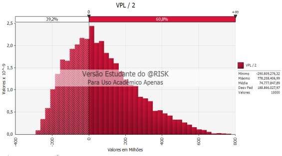
Graph 5 - Simulation distribution plot using @RISK
Source: Authors. (Out, 2019)
Graph 6 - Simulation tornado graph using @RISK
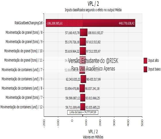
Graph 6 - Simulation tornado graph using @RISK
Source: Authors. (Out, 2019)
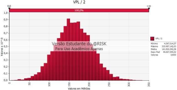
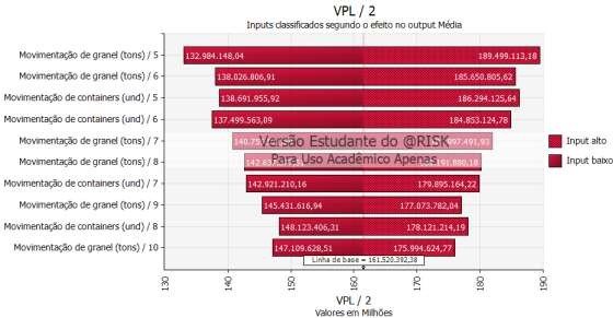
Thus, with the use of the program's "achieve goal" tool, we can see what rate would make the project 100% viable, thus eliminating one of the most worrying variables of the project. In this case, the best rate of return was 13%, its minimum profit would be R$ 31,037,395.49 and the maximum of R$ 339,958,347.32, with an average of R$ 165,003,970, 68 and standard deviation of R$ 39,962,553.4, where the standard deviation is below the mean, meaning that there is a low variability of the values and that despite this variability the values are still positive. In this scenario, the tornado graph (Graph 6) will show which event and in which year will have the greatest impact on the NPV (net present value), observed in the graph that the movement of solid bulk in the seventh and eighth year of the project are the main variables, and the distribution graph (Graph 5) shows that this project is fully viable at the established rate.
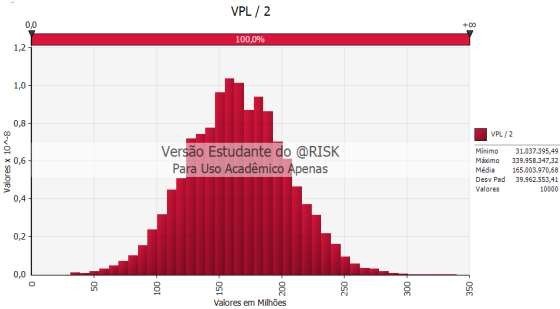
Graph 7 - Distribution chart with “Achieve Goal” function using @RISK
Source: Authors. (Out, 2019)
Graph 8 - Tornado chart with “Reach Goal” function using @RISK
Source: Authors. (Out, 2019)
With the previously used order of construction of the terminals for the analysis, the project presented a risk of 60.8%, considering the rate as a variable. The order of construction of the terminals was changed, positioning the containers and solid mineral bulk to be built first and then the fuel and agricultural bulk terminals. After the changes in the spreadsheet, new graphics were generated with the program under the same conditions as the previous ones, with the rate varying from 10% to 18%. Graph 7 shows that the project now presents a viability percentage of 92,3%, making more viable when compared to the previous scenario, with a difference of 31,5%, and a standard deviation close to the mean, explaining why the high rate of project viability in this scenario.
Graph 9 - Scenario 2 distribution plot using @RISK
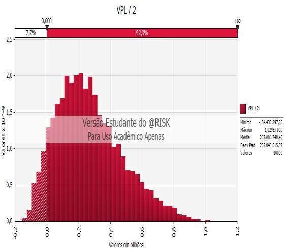
Graph 9 - Scenario 2 distribution plot using @RISK
Source: Authors. (Out, 2019)
After using "achieve goal" in this case, we obtained graph 8, which is a distribution graph declaring that the project is 100% viable within the rate calculated by the program, which was 14.7%, 1.7% higher than the 1st case.
Graph 10 - Scenario 2 distribution chart with the “Achieve Goal” function using @RISK
Source: Authors. (Out, 2019)
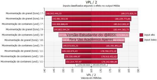
In the tornado graph (Graph 9), there was a change in the order of each movement annually, showing in this case that the variation of bulk movement in years 5 and 6 is the one that contains the greatest risk for the project's NPV and, afterwards, the container movement in year 5.
Graph 11 - Scenario 2 tornado graph with the “Reach Goal” function using @RISK
Source: Authors. (Out, 2019)
5. CONCLUSION
The objective of this work was to carry out a risk analysis of the implementation of an offshore port, located in the north of the State of Pará.
The first step was to develop a risk model from the data collected, where the importance for the development of this model was highlighted and from which it was possible to identify the variation in the movement of containers used to execute the risk model at its worst case of 500,000 units, in the best case with 2,500,000 units and the fixed value for the model of 1,500,000 units. together with the fixed values of solid and liquid bulk, obtained by the average of movements in tons per year in the ANTAQ’s yearbook of the northern region, with an average for solid bulk of 60,000,000 tons, worst case of 40,000,000 tons and best case of 80,000,000 tons, for liquid bulk the average was 15,500,000 tons, worst case 13,000,000 tons and best case 17,000,000 tons.
With the data obtained and inserted in the risk model, it was possible to carry out the risk analysis through the @RISK software and evaluate the feasibility of implementing the port project, where it was observed that the project is 100% viable after using the tool " achieve goal”. In the first case, the rate of return to achieve this result was a maximum of 13% and in the third case it was 14.7%. It was possible to observe that the change in the order of construction of the terminals, starting with the mineral bulk and container terminals, made the project with a lower risk of being unfeasible during its 35 years of implementation. The results demonstrate through the financial and economic risk analysis that the offshore port in the northern region of Brazil becomes viable.
Based on the fourth case, where the best results for the project were obtained, due to the change of terminals and use of the tool "achieve goal", it was possible to observe in the tornado graph the greatest risks to the net present value of the project, highlighting the great risk of bulk handling in the fifth and sixth year, container handling in the fifth and sixth year, bulk handling in the seventh and eighth year. From these data, it is observed that the main risks of the project are focused on the movement of solid bulk and containers, therefore, an action plan is necessary to contain these variations in values and create safeguards.
Since all the objectives proposed for this work were achieved and considering that it is possible to change the schedule, the variables, the number of simulations etc., thus making it possible to observe the worst and best scenario, in addition to demonstrating the possible risks and its degree of importance during the first 35 years simply by changing some factor to analyze what happened to the project after that change.