Methods of Finite Differences in the Domain of Time Applied to the Equation of Heat Biotransfer in Ocular Tissues

1. Introduction

Over the years, several numerical and applied applications to engineering to analyze and solve problems in medicine and particularly involving heat transfer, which is the area of interest of this article. These tools are employed through numerical simulation methods of physical and biological phenomena.

An example of this is laser surgeries, which have been increasing their applications because of their positive results, using the fundamental principles of heat transfer. Hypothermic treatments are used to destroy cancerous lesions, for example. Consequently, many therapies and medical devices operate by destructively heating or cooling diseased tissue while leaving adjacent healthy tissue undisturbed. With the growing advances in biomedical engineering, many medical devices have been developed that aid treatments, such as the destruction of eye tumors. These devices or tools must be developed to control the distribution of temperatures throughout the heat treatment and the distribution of chemical species in chemotherapy (Guimarães, 2003; Incropera, 1976).

With the study of the Bioheating Transfer Equation - BHTE, it is possible to analyze and develop tools that help in these treatments. BHTE is the heat conduction equation, with one term added to the equation, and this specific term is heat generation due to blood perfusion. The BHTE can be used to verify and analyze the temperature variation in the human eye before surgery that uses, for example, a laser as a surgical instrument or during any hyperthermic procedure (Silva, 2004).

This article analyzes temperature variation in biological tissues

using a two-dimensional model of a human eye. The technique employed used the finite difference method in the time domain, which allowed heat transfer analysis due to irradiation from an external source. In addition to analyzing the thermal damage caused by the source.

 

2. Materials and methods

According to (CHAPRA, 2013) numerical methods are tools mathematics by which mathematical problems are formulated so that they can be solved with arithmetic operations. There are many numerical methods, such as the energy balance method, the boundary element method, the finite element method and the finite difference method. The methods mentioned have one feature in common: they all involve a large number of arithmetic calculations. And all of them can be used in Heat Biotransfer problems. The method chosen for this work is the finite difference time domain (FDTD) method. The FDTD method is very effective in this type of analysis, as it shows it in a simple way, without much computational effort compared to others.

With the advances and development of computers, these methods are widely used as computers can solve these problems faster and more efficiently. It is resulting in the increased use of these methods for simulation in engineering. With the help of software such as Matlab, it is possible to develop an algorithm that describes the problem to be solved, creating a routine iteratively, so that these calculations can be repeated several times until reaching the desired precision; in addition, we can plot graphs of the problem that can be generated in a simple way, in the same interface of the software.

 

2.1 Description of the Mathematical Model

The heat biotransfer equation is a heat conduction equation, with a specific term for heat generation due to added blood perfusion. The analysis considers the effect of the heat pulse on living tissue — estimates of parameters of the Pennes equation (Guimarães, 2003).

In his work, Harry H. Pennes (1948) proposed an equation that describes heat transfer in human tissues and organs, including the effects of blood flow through the heat biotransfer equation. The linear mathematical model obtained in this study represents the energy balance within biological tissues through the interaction of blood perfusion and metabolism.

Equation 1 represents the Pennes heat biotransfer equation:

 

(1.0)

 

Where:

	tissue thermal conductivity;
	tissue density;
	tissue specific heat;
	temperature;
	time
	heat source due to blood perfusion;
	heat source due to metabolic heat generation;
	heat source due to blood perfusion;

 

A term in the equation will need to be neglected because, according to (Sturesson & Andersson-Engels, 1995), generally, the generation of metabolic heat  is much smaller than the external heat deposited, in our case, the laser. Also, the heat source due to perfusion is given by ; that is, it is like removing the heat due to the capillary vascularization present in the tissues. This term can be represented by equation 2 (Diller, 1992):

 

(2.0)

 

Where:

	volumetric blood perfusion rate;
	blood specific mass;
	specific heat of the blood;
	temperature of arterial blood entering tissue;
	temperature of the venous blood leaving the tissue.

The blood temperature is not the same at each point of the tissue. According to (Guimarães, 2003) the temperature of the blood that enters the capillary region is equal to the temperature of the arterial blood and the temperature of the blood that leaves is the temperature of the venous blood, , which can be considered the same as the local temperature  of the tissue. The velocity of blood in the capillaries is minimal, with a Peclet number (which expresses the relationship between heat transfer by convection and heat transfer by conduction) much less than unity. This fact justifies the consideration that the temperature of the venous blood leaving the tissue is equal to the temperature of the latter.

Replacing the  by  at the local temperature. Soon  becomes:

 

(3.0)

 

This blood perfusion rate cannot be measured directly (Charny, 1992), making it difficult to obtain values closer to real values for different types of tissues. Therefore, to arrive at acceptable values, as well as tissue properties in vivo, it is necessary to analyze before removal.

Thus separating the effects of blood flow and metabolic heat generation so that the thermal properties of the medium can be deduced.

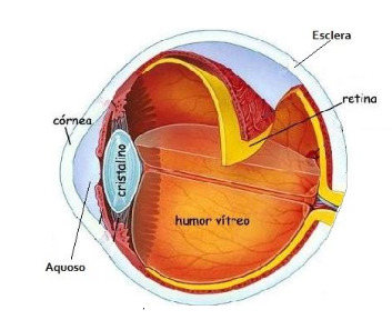
Assuming that heat transfer occurs by convection between the corneal surface and the external environment; internal driving; and convective heat transfer from the retina to the choroid due to blood flow in this region. Therefore, considering the specifications of these parameters that we will use from now on, the eye is represented by six specific areas with different thermophysical properties: the cornea, the aqueous, the lens or lens, the vitreous, and the retina, as shown in figure 1. (Silva, 2004).

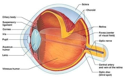
Figure 1 - Cross-section scheme of the human eye. Source: Google Images

 

Ocular biological tissue has a certain degree of sensitivity, as the most of them contain a large percentage of aqueous liquid. However, if they are exposed to high temperatures, thermal damage can occur. That is, it can cause first, second, and third-degree burns. The process of thermal tissue damage occurs with the denaturation of proteins, thus losing their biological activity. Therefore, irreversible destruction of living tissue can occur (Diller, 1992). For example, these effects may be due to significant heat sources, which in the proposed case is laser irradiation.

Several researchers have made the first quantitative assessments of damage or burning in living tissue. Most of these experiments were done on animal tissue or human skin to determine the temperature-time exposure relationship to create various classifications of damage levels. With these data, it was possible to describe the thermal damage as a process rate dependent on temperature. It can be observed that the increase in damage occurs as an exponential proportion to the absolute temperature (Diller, 1992).

In this work, we will analyze the temperatures in order not to cause irreversible damage. Because, some analyzes, such as the one given by (Rol, 2000), indicate that it only starts to suffer thermal damage and protein denaturation from 37°C onwards. And Second (Diller, 1992), irreversible thermal tissue damage occurs at temperatures between 65°C and 75°C.

The model by Henriques and Moritz (1947) was used because they were one of the first researchers to present a quantitative model to assess thermal damage in biological tissues, even if it is an in vitro experiment, with animal and human skin. They related thermal tissue damage as an integral part of a chemical process and used an Arrhenius-type equation to exemplify the damage mathematically.

 

(4.0)

 

Where:

	scalar constant
	reaction activation energy
	universal gas constant
	absolute temperature
	time

 

2.1.1 Mathematical Modeling

 

The finite difference method (FDM) is used to calculate the partial derivatives present in differential equations. The technique replaces each derivative or differential of the differential equations with numerical approximations of the same order of approximation using the Taylor Series. (CHAPRA,2013).

Taylor series expansion:

 

(5.0)

 

As the central derivative, obtained through the arithmetic mean of the other two derivatives, it is given by:

 

(6.0)

 

The numerical methods replace the differential equation of heat conduction with a set of  algebraic equations for unknown temperatures at  points strategically chosen in the middle. The simultaneous solution of these equations results in the temperature values at these points discreet.

The first derivative of  at the midpoint is equivalent to the slope of the line tangent to the curve at this point, defined as:

 

(7.0)

 

Thus, the ratio between the ∆𝑓 increment of the function and the ∆𝑥 increment of the independent variable, when ∆𝑥 → 0. If we do not take the indicated limit, we will have the following approximate relationship for the derivative:

 

(8.0)

 

 

This expression is the finite difference form of the first derivative. The same equation can also be obtained by writing the Taylor series expansion of the function 𝑓 over the point 𝑥,

 

(9.0)

 

And the second derivative of 𝑓(𝑥) at the midpoint is equivalent to the slope of the line tangent to the curve at that point, defined as:

(10.0)

 

2.1.2 Finite Difference Method

Two-dimensional problems involving geometries or boundary conditions are mostly complex; we can't develop solutions by analytical methods so quickly. Therefore, in this work, we chose to use the numerical methods, in our case, the finite difference method in the time domain.

The numerical solution allows the determination of temperature only

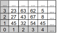
discrete points, unlike the analytical solution that determines the temperature at any point of interest in the medium. The first step in numerical analysis is the selection of these points. For this, we should look at Figure 2, which shows how this can be done by subdividing the medium of interest into a series of small regions and specifying for each a reference point located at its center.

The reference point is often called a nodal point (or simply a node), and the aggregate of points is called a nodal network (or mesh). The nodal points are identified by a numbering scheme which, for a two-dimensional system, can take the form shown in Figure 2. The  and  positions are identified by the indices  and , respectively.

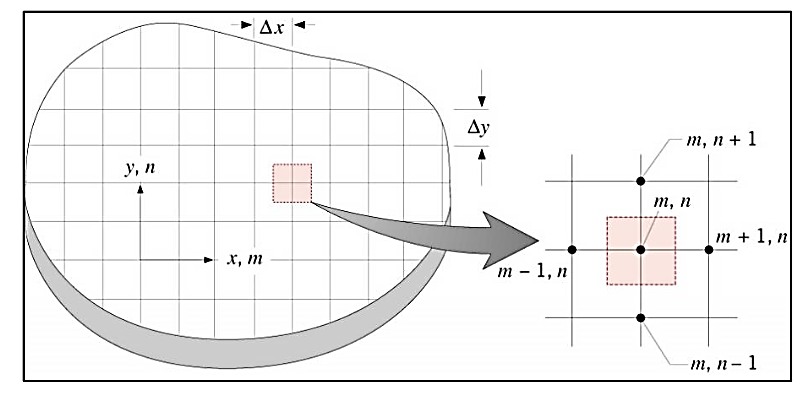
Figure 2. Nodal mesh. Source: Incropera

 

Since each node represents a specific region and its temperature is a measure of the region's average temperature. For example, the temperature of node  in Figure 2 can be seen as the average temperature of the adjacent shaded area. Since the selection of points is rarely random, depending on aspects such as geometric convergence and desired precision.

The numerical accuracy of the calculations strongly depends on the number of nodal points used. If this number is large, the solutions will be more accurate.

The numerical determination of the temperature distribution requires that an appropriate conservation equation is written for each of the nodal points of unknown temperature.

The resulting set of equations must then solve the resulting equation set simultaneously for the temperatures at each node.

For any interior node in a two-dimensional system with no generation and uniform thermal conductivity, the exact form of the energy conservation requirement is given by the heat biotransfer equation, which is the heat equation with the energy generation term heat by blood perfusion.

However, if the system is characterized in terms of a nodal network, it becomes necessary to work with an approximate, or finite difference, form of this equation.

Thus, the finite difference equation suitable for the internal nodal points of a two-dimensional system can be deducted directly from the heat biotransfer equation:

 

(11.0)

 

Thus,

 

(12.0)

 

Metabolic heat is neglected as it is much smaller than the external heat source . Then:

 

(13.0)

 

Where the diffusivity α, is given by:

 

(14.0)

 

Making the necessary replacements:

 

(15.0)

 

And applying finite differences, the second derivative of 𝑓(𝑥):

 

(16.0)

 

Equation (16.0) represents the steady state heat biotransfer equation.

To obtain the form of finite differences in the time domain, we need to make some considerations. As we saw earlier, we can use the central difference approximations for the spatial derivatives represented by equation (16.0).

Using the subscript indices  and  can designate the positions of discrete nodal points in relation to the  and  axes. However, in addition to being discretized in space, the problem must also be discretized in time. The integer p is introduced for this purpose, where:

 

(17.0)

 

And the finite difference approximation for the derivative concerning time in equation 16 is represented by:

 

(18.0)

 

The superscript index p is used to indicate the temporal dependence of the temperature T, and the derivative concerning time is expressed in terms of the difference between the temperatures associated with the new (p + 1) and previous (p) instants time.

Thus, must perform the calculations at successive time instants separated by time interval ∆𝑡.

Just as the solution of finite differences in space is limited to determining the temperature at discrete points, it also restricts temperature determination to discrete points in time.

Replacing equation 16 into  into equation 18, in the explicit form of the finite difference equation for the internal node  and  is:

 

(19.0)

 

Explaining the nodal temperature at the new instant of time  and considering that ∆𝑥 = ∆𝑦, we have to:

 

(20.0)

 

Where  is a finite difference form of the Fourier number, relationship between the rate of heat conduction and the accumulation of thermal energy in a solid, being a dimensionless number.

 

(21.0)

So that the finite difference method does not converge, we must adopt a stability criterion:

(22.0)

 

Convergence means that when x and t tend to zero, the results of the finite difference technique approach the true solution.

Stability means that errors at any stage of the calculation are not amplified but attenuated as the progress of the analysis.

Therefore, the  must be less than a quarter of the ratio of the square of the mesh pitch and the thermal diffusivity of the fabric.

 

2.1.3 Implementation and Computational Modeling

With the physical-mathematical model developed and with the described equations that govern the domain of the object of study, including knowledge of the constitutive models and parameters of the parts that form it, the computational model to be used in the simulation must be built. And in turn, with the application of

heat biotransfer equation in the simulation of biological systems, which will be subject to the most varied thermal procedures, requires great geometric flexibility in all stages of the adopted computational modeling

(GUIMARÃES, 2003).

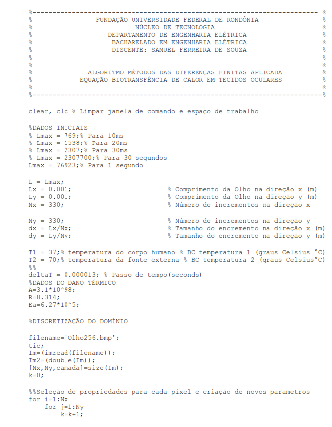
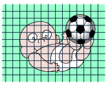
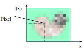
To start such an implementation, we need to discretize the domain. We will use image processing because a digital image is obtained from the sampling and quantization of a function. A function  can be represented, only in this case,  and  are integers. Once the plane is sampled, we have various values representing the color. Each element of this array is called a Pixel.

Figure 3 illustrates the image discretization process and shows a possible color coding for each element of the matrix.

 

Figure 3. Discretization of an Image Process. Source: Scuri,2002.

 

In these images, the pixel value contains a single number corresponding to an index for the table, including the color value in RGB (Red, Green, Blue), according to the table in Figure 3. The three components are reduced to 1. Table 1 shows the index mapping of the Color Table.

 

Table 1. Index Mapping in Color Table

 

Image		Color Table Index R G B

The pixels are normally square, generating a regular grid due to evenly spaced sampling, we can compare with the nodal network.

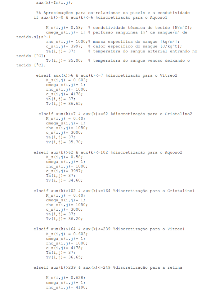
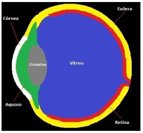
Using the Matrix Laboratory - Matlab software, the six main parts of the eye with different thermophysical properties were discretized: the cornea, the aqueous humor, the crystalline or crystalline, the vitreous humor, the sclera and the retina, as shown in Figure 5.

(a)		(b)
Figure 5. (a) . Source: Google Image,2022 (b) . Source: Author

 

After finishing the discretization of the image with the standard colors, a matrix of 350x350 pixels is generated with colors and their respective numbers shown in Table 2.

 

Table 2. Color Table
Color	Number
Black	0
Red	79
Green	113
Gray	164
Blue	210
Yellow	251
White	255
Source: Author

 

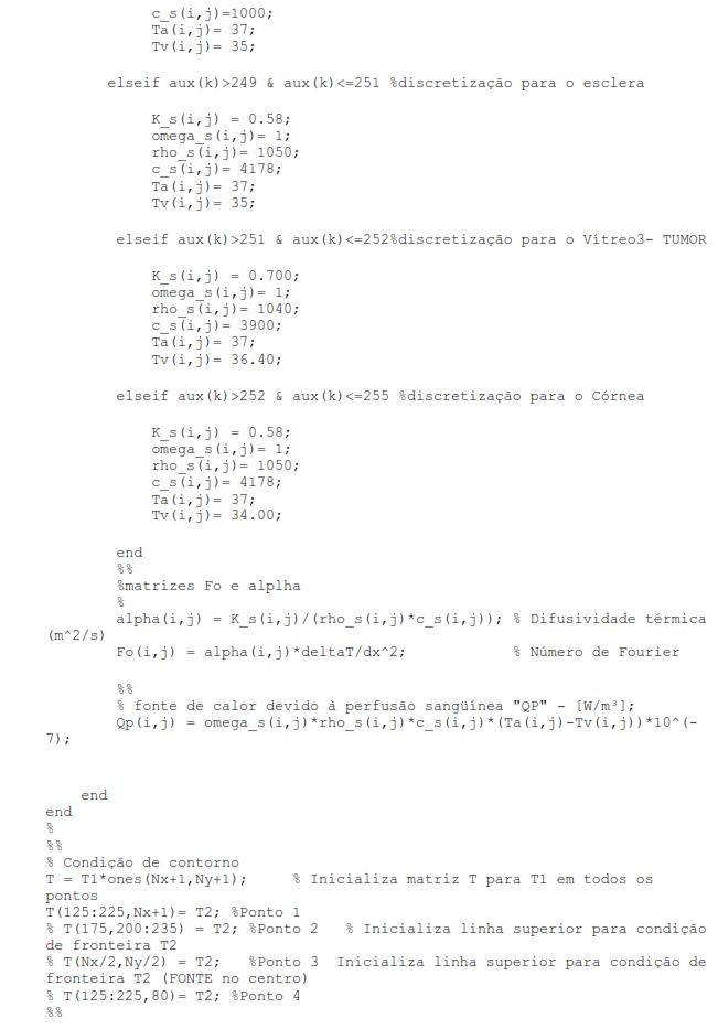
The modeling procedure used in the study of bioheat transfer comprises the following steps: image discretization; geometric modeling and generation of discrete matrices; data pre-processing; numerical analysis program via Finite Differences Method; post-processing and visualization of results.

The analysis used the Finite Differences Method implemented in Matlab language with a microcomputer with Intel i7 3 GHz processor with 4GB of RAM.

Thermal properties of various components in the human eye are listed in Table 3.

 

Table 3.  Thermal properties of various parts of human eye

Eye tissue	Property
	Thermal conductivity K[Wm-1K-1]	Specific heat capacity C [JKg-1K-1]	Density ρ[kgm-3]
Cornea	0.580	4178	1050
Aqueous humor	0.578	3997	7 1050
Lens	0.400	3000	1000
Iris	1.680	3650	1100
Vitreous humor	0.594	3997	1000
Retina	0.565	3680	1000
Sclera	0.580	4178	1000
Blood	0.530	3600	1050
Source: Mirnezami SA, Rajaei Jafarabadi M, Abrishami M., 2013

 

The analytical solution of the Penne bioheat transfer equation is limited to some simple geometries with a high degree of symmetry. Still, using the Finite Element Method, we adopt the following considerations:

1. Heat transfer within the eye occurs by conduction;
2. Not considered a calorie generation ;

• Blood perfusion was not considered;

1. The initial temperatures in the different regions of the eye were obtained through the study of (Amara, 1995);
2. Blood temperature is considered to be .

The eye will be represented by six regions of different thermophysical properties: the cornea, the aqueous humor, the lens or crystalline, the vitreous humor, the sclera, and the retina.

The boundary conditions and initial conditions are:

1. Convective heat transfer between the corneal surface and the external environment;
2. Convective heat transfer between the retina and the choroid.

The initial temperatures of certain regions will be adopted second (Amara, 1995) with subdivisions in the vitreous, crystalline, aqueous. Also, we consider the sclera part of the vitreous humor as it has similar characteristics. The following table 4 presents the initial temperatures. The blood temperature is taken equal to 37°C. The ambient control temperature was considered constant and equal to 20°C.

 

Table 4. Temperature without heat source

Fabric	Temperature
Retina	36.90
Vitreous 1	36.85
Vitreous 2	36.65
Vitreous 3	36.40
Crystalline 1	36.20
Crystalline 2	35.70
Aqueous 1	35.00
Aqueous 2	34.60
Cornea	34.00

Source: Amara, 1995

 

The dimensions of the human eye were obtained from the work of Amara (1995) and Gokul (2013), as shown in Figure 6. We also consider that the sclera is part of the vitreous because it has similarities in its characteristics. Measurements were made from the central axis to its specific regions, as shown in Figure 5b, resulting in Table 5. In this way, we divided the vitreous into three parts, the crystalline into two and the aqueous into two, as shown in Figure 7.

 

Table 5. Eye Dimension

Fabric	Dimension
Cornea	0.0005
Aqueous	0.0035
Crystalline	0.0070
Vitreous	0.023
Retina	0.025
Source: Author

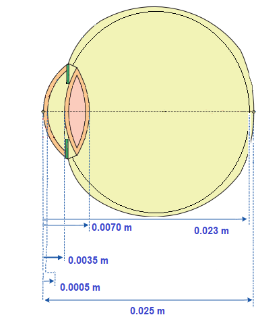
Figure 6. . Source: Gokul (2013)

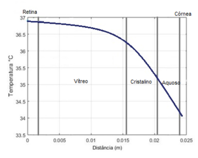
Figure 7. .

Source: Author

 

The reference model is a physical system described by equivalence differences consisting of the heat equation that includes the laser heat source and the threshold and initial condition equations.

The analytical system is transformed into an integral formulation where a Galerkin function is applied. Finite element method to drive a discrete algebraic system solved by numerical methods.

The method used in this work is based on the discretization of an RGB image later transformed into a matrix of integers, transforming it into an algebraic system, thus inserting thermophysical properties and solving by the numerical method of finite differences. We will consider temperature control from  to .

The transfer of heat in a biological tissue occurs more slowly because it has a large amount of water in its composition, causing heat propagation in the tissue to have a very long simulation time since their characteristics vary. After all, they have several different types of fabrics and with different temperatures.

We applied an external source at a temperature of  and used 1 second since most heat sources for surgery use the time interval from  to . The numerical approach is based on equation (20). Numerical simulation parameters are shown in table 6.

Then, spacings of  were adopted in both x and y, which implies a time step of  equal to . By the stability, criterion  must be less than a quarter of the ratio between the square of the mesh pitch and the thermal diffusivity of the fabric.

 

Table 6. Simulation parameters
Source: Author

 

The heat propagation depends on the thermal diffusivity of the fabric because the higher the heat transfer, we can see from equation (14).

As for the ocular tissues, the thermal diffusivity varies between  to     making the heat transfer occur more slowly, so we need large time steps for the simulation to be more accurate.

Table 7 shows the differences in thermal diffusivity between materials and fabrics. And Figure 8 presents the position of the heat source and the points for the output graph.

 

Table 7. Thermal diffusivity table
Thermal Diffusivity
Copper
Nickel
Fabric (Vitreous)
Water
Source: Author

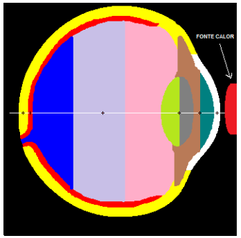
Figure 8. . Source: Author

 

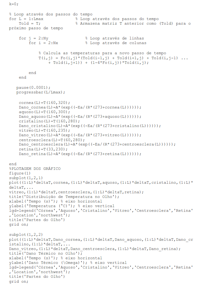
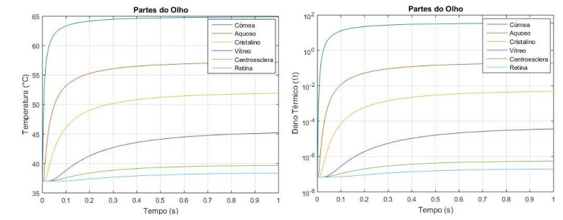
The graph shown in Figure 9a shows the point in the corneal region, where the temperature only starts to increase after  (milliseconds), applying the external source with a temperature of . The graph shown in Figure 9b shows the thermal damage done to the tissue in approximately . The simulation presented values very close to the literature, demonstrating the method's functionality. The temperature is the same in the sclera until it reaches  because it is further away from the heat source. And because their thermophysical characteristics are different. Also, it did not suffer thermal damage; we can observe that the temperature does not suffer many variations. Aqueous humor is composed of large amounts of water and protein, and the graph shown in Figure 9b shows that conduction happens quickly but does not cause damage due to its composition. In the lens, because it has a smaller thickness than the other eye regions, the temperature variation is low compared to the other parts. Figure 9b showing the thermal damage graph, shows that there is not enough change to cause a burn in this region.

The vitreous humor consists of a transparent gel with hydration of approximately , and it is two to four times more viscous than water. Also, due to its greater thickness and composition in liquid form, the temperature variation only occurs at about . Not suffering any thermal damage because of the low-temperature variation in the region.

The retina is the outer part of the eye, so the heat transfer took place over a more extended period, even though the thickness was small. Most diseases of the human eye affect this specific part. The region in the simulation did not suffer any thermal damage because it was far from the source with a slight temperature variation.

• (b)

Figure 9 (a) (b) Graph of Thermal Damage

Tissue damage is defined as the denaturation of proteins or the loss of biological functions of molecules found in cells or in extracellular fluids (Diller, 1992). This thermal damage can occur when tissue temperature exceeds the range within which normal life processes exist. High and low temperatures can cause irreversible changes in molecules, resulting in thermal damage. Typical examples are burns and skin frostbite. The most successful mathematical models consider that thermal damage is a chemical reaction that depends on the temperature and the time interval to which the living tissue was subjected. The models describe the effect of heat on the chemical reaction rate and consider the variation in the concentration of undamaged molecules using Arrhenius' law. Although the meaning of the thermal damage function is not very well defined, it was considered that when the damage function assumes the value one , which corresponds to approximately  of the denatured proteins, complete necrosis, or damage, occurred. Irreversible damage to biological tissue (Henriques and Moritz, 1947).

 

3. Conclusion

Considering the observations described in this work, we can conclude that it is possible to determine thermal damage in ocular tissues using the time domain differences method with few thermophysical characteristics of the eye.

The results presented were very close to the literature. It evidences the possibility of developing a tool that helps in the two-dimensional modeling of the human eye with bioheat transfer analysis.

Although, several works have pointed out challenges such as the lack of information about the natural values of the physical parameters of eye tissues due to the need for in vivo experiments. The simulation was able to show the behavior of temperature variation in the human eye. Given the results achieved for future research, treat the problem in three dimensions and implement an error estimator to control the stability of the proposed method.

Appendix 1